Utilities
Dij Matrix
- _steepness.get_Dij(self) ndarray
Function to get Dij Matrix (Corrected version for chance)
Parameters
Returns
- dij_matrixnp.ndarray
Dij matrix, the initial order of the matrix kept intact and resulting corrected dominance indices (rounded to 4 decimal places)
See also
https://numpy.org/doc/stable/reference/generated/numpy.divide.html
Notes
When estimating A’s chances of defeating B we have to take the number of interactions into account. To this purpose proposed a dyadic dominance index dij in which the observed proportion of wins, Pij, is corrected for the chance occurrence of this observed outcome. de Vries proposed calculating the chance occurrence of the observed outcome on the basis of a binomial distribution with each animal having an equal chance of winning or losing in every dominance encounter. In the present paper we propose calculating the chance occurrence of the observed outcome on the basis of a uniform distribution, that is, given a certain number of observed dominance encounters, nij, then by chance every possible division of these encounters in wins and losses among the two animals is equally likely. (de Vries, 2006)
References
de Vries H, Stevens JMG, Vervaecke H (2006). “Measuring and testing the steepness of dominance hierarchies.” Animal Behaviour, 71, 585-592. doi: 10.1016/j.anbehav.2005.05.015.
Example:
 1mat = np.array([[0, 58, 50, 61, 32, 37, 29, 39, 25],
 2                [8, 0, 22, 22, 9, 27, 20, 10, 48],
 3                [3, 3, 0, 19, 29, 12, 13, 19, 8],
 4                [5, 8, 9, 0, 33, 38, 35, 32, 57],
 5                [4, 7, 9, 1, 0, 28, 26, 16, 23],
 6                [4, 3, 0, 0, 6, 0, 7, 6, 12],
 7                [2, 0, 4, 1, 4, 4, 0, 5, 3],
 8                [0, 2, 1, 1, 5, 8, 3, 0, 10],
 9                [3, 1, 3, 0, 0, 4, 1, 2, 0]])
10name_arr = np.array(["V", "VS", "B", "FJ", "PR", "VB", "TOR", "MU", "ZV"])
11hier_mat = Hierarchia(mat, name_arr)
12dij_matrix = hier_mat.get_Dij()
13print(dij_matrix)
Result:
[[0.     0.8731 0.9352 0.9179 0.8784 0.8929 0.9219 0.9875 0.8793]
 [0.1269 0.     0.8654 0.7258 0.5588 0.8871 0.9762 0.8077 0.97  ]
 [0.0648 0.1346 0.     0.6724 0.7564 0.9615 0.75   0.9286 0.7083]
 [0.0821 0.2742 0.3276 0.     0.9571 0.9872 0.9595 0.9559 0.9914]
 [0.1216 0.4412 0.2436 0.0429 0.     0.8143 0.8548 0.75   0.9792]
 [0.1071 0.1129 0.0385 0.0128 0.1857 0.     0.625  0.4333 0.7353]
 [0.0781 0.0238 0.25   0.0405 0.1452 0.375  0.     0.6111 0.7   ]
 [0.0125 0.1923 0.0714 0.0441 0.25   0.5667 0.3889 0.     0.8077]
 [0.1207 0.03   0.2917 0.0086 0.0208 0.2647 0.3    0.1923 0.    ]]
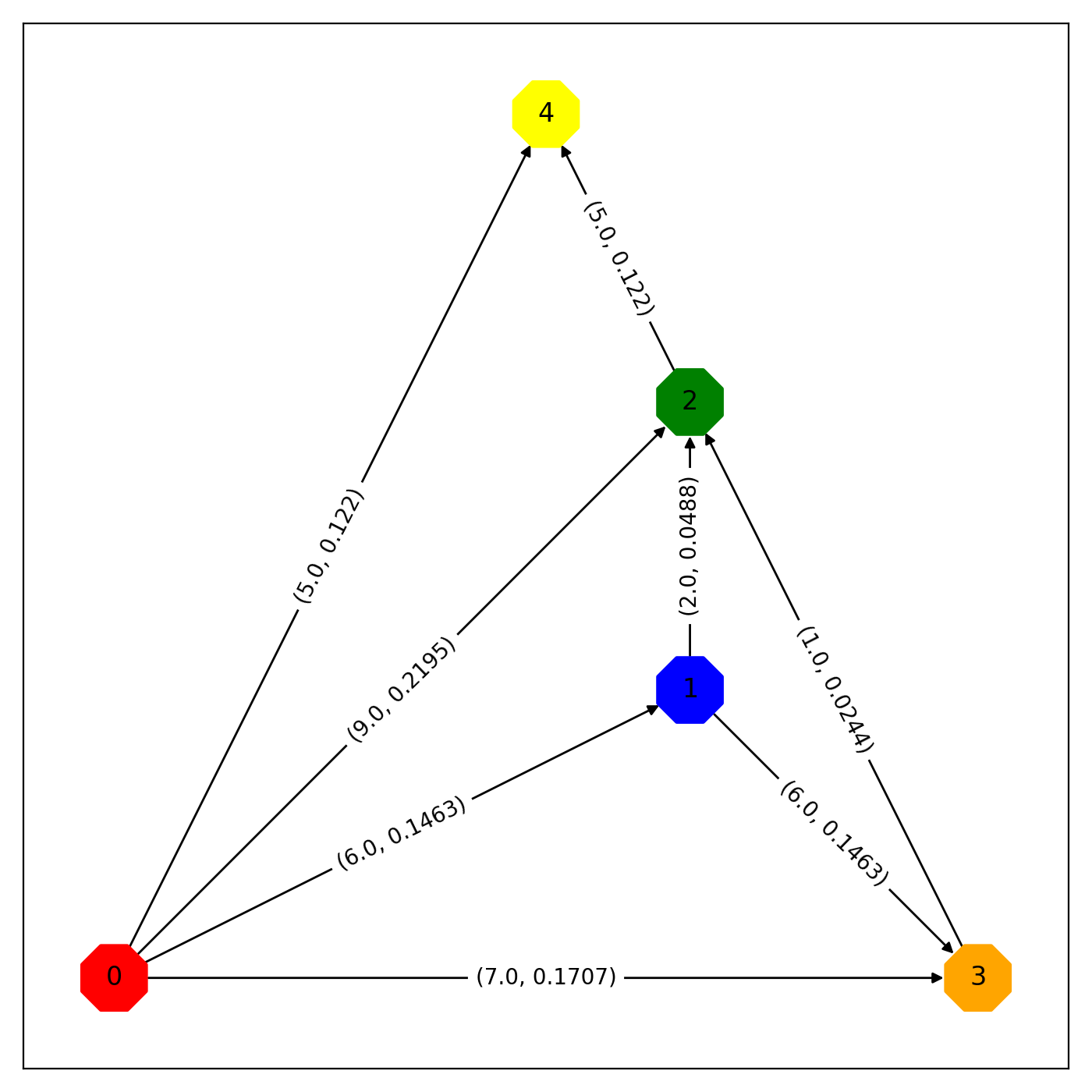
Directed Network Plot (Planar Layout)
- _network_graph.directed_network_graph(self, **kwargs) Figure
Directed network graph with absolute and proportional win tuples in edges.
Parameters
- param kwargs:
dict Pass parameter for fig_size in matplotlib and pass parameters for draw_networkx method.
Returns
- figurematplotlib.figure.Figure
Planar layout network graph figure. The nodes are named as indices passed to Hierarchia object. The edges have absolute and proportional dyadic relationship indicators.
See also
https://networkx.org/documentation/stable/reference/classes/digraph.html https://networkx.org/documentation/stable/reference/generated/networkx.drawing.layout.planar_layout.html https://networkx.org/documentation/stable/reference/generated/networkx.drawing.nx_pylab.draw_networkx.html
Example:
1mat = np.array([[0, 6, 9, 8, 5],
2                [0, 0, 4, 6, 0],
3                [0, 2, 0, 4, 7],
4                [1, 0, 5, 0, 3],
5                [0, 0, 2, 3, 0]], dtype='float32')
6hier_mat = Hierarchia(mat)
7fig = hier_mat.directed_network_graph(fig_size=(7, 7),
8                                      node_color=['red', 'blue', 'green', 'orange', 'yellow'],
9                                      font_size=12)
Result: